# load packages
library(tidyverse)   # for data wrangling and visualization
library(tidymodels)  # for modeling
library(usdata)      # for the county_2019 dataset
library(openintro)   # for Duke Forest dataset
library(scales)      # for pretty axis labels
library(glue)        # for constructing character strings
library(knitr)       # for neatly formatted tables
library(kableExtra)  # also for neatly formatted tablesf


# set default theme and larger font size for ggplot2
ggplot2::theme_set(ggplot2::theme_bw(base_size = 16))SLR: Permutation test for the slope
Announcements
HW 01 due Tuesday, January 28 at 11:59pm
Labs resume on Monday
Topics
Evaluate a claim about the slope using hypothesis testing
Construct a null distribution using simulation
Define mathematical models to conduct inference for slope
Computational setup
Recap of last lecture
Data: Duke Forest houses
The regression model
df_fit <- lm(price ~ area, data = duke_forest)

tidy(df_fit) |>
kable(digits = 2)| term | estimate | std.error | statistic | p.value |
|---|---|---|---|---|
| (Intercept) | 116652.33 | 53302.46 | 2.19 | 0.03 |
| area | 159.48 | 18.17 | 8.78 | 0.00 |
. . .
Slope: For each additional square foot, we expect the sale price of Duke Forest houses to be higher by $159, on average.
Inference for simple linear regression
Calculate a confidence interval for the slope, \(\beta_1\)
Conduct a hypothesis test for the slope, \(\beta_1\)
Statistical inference
Sampling is natural

- When you taste a spoonful of soup and decide the spoonful you tasted isn’t salty enough, that’s exploratory analysis
- If you generalize and conclude that your entire soup needs salt, that’s an inference
- For your inference to be valid, the spoonful you tasted (the sample) needs to be representative of the entire pot (the population)
Confidence interval via bootstrapping
- Bootstrap new samples from the original sample
- Fit models to each of the samples and estimate the slope
- Use features of the distribution of the bootstrapped slopes to construct a confidence interval
Bootstrapping pipeline I
Response: price (numeric)
Explanatory: area (numeric)
# A tibble: 98 × 2
price area
<dbl> <dbl>
1 1520000 6040
2 1030000 4475
3 420000 1745
4 680000 2091
5 428500 1772
6 456000 1950
7 1270000 3909
8 557450 2841
9 697500 3924
10 650000 2173
# ℹ 88 more rowsBootstrapping pipeline II
Response: price (numeric)
Explanatory: area (numeric)
# A tibble: 98,000 × 3
# Groups: replicate [1,000]
replicate price area
<int> <dbl> <dbl>
1 1 290000 2414
2 1 285000 2108
3 1 265000 1300
4 1 416000 2949
5 1 541000 2740
6 1 525000 2256
7 1 1270000 3909
8 1 265000 1300
9 1 815000 3904
10 1 535000 2937
# ℹ 97,990 more rowsBootstrapping pipeline III
set.seed(210)

duke_forest |>
specify(price ~ area) |>
generate(reps = 1000, type = "bootstrap") |>
fit()# A tibble: 2,000 × 3
# Groups: replicate [1,000]
replicate term estimate
<int> <chr> <dbl>
1 1 intercept 80699.
2 1 area 168.
3 2 intercept -18821.
4 2 area 205.
5 3 intercept 234297.
6 3 area 117.
7 4 intercept 134481.
8 4 area 150.
9 5 intercept 23861.
10 5 area 190.
# ℹ 1,990 more rowsBootstrapping pipeline IV
Visualize the bootstrap distribution

Compute the CI
But first…
obs_fit <- duke_forest |>
specify(price ~ area) |>
fit()
obs_fit# A tibble: 2 × 2
term estimate
<chr> <dbl>
1 intercept 116652.
2 area 159.Compute 95% confidence interval
boot_dist |>
get_confidence_interval(
point_estimate = obs_fit,
level = 0.95,
type = "percentile"
)# A tibble: 2 × 3
term lower_ci upper_ci
<chr> <dbl> <dbl>
1 area 91.7 211.
2 intercept -18290. 287711.Hypothesis test for the slope
Research question and hypotheses
“Do the data provide sufficient evidence that \(\beta_1\) (the true slope for the population) is different from 0?”
. . .
Null hypothesis: there is no linear relationship between area and price
\[ H_0: \beta_1 = 0 \]
. . .
Alternative hypothesis: there is a linear relationship between area and price
\[ H_a: \beta_1 \ne 0 \]
Hypothesis testing as a US court trial
- Null hypothesis, \(H_0\): Defendant is innocent
- Alternative hypothesis, \(H_a\): Defendant is guilty
- Present the evidence: Collect data
- Judge the evidence: “Could these data plausibly have happened by chance if the null hypothesis were true?”
Yes: Fail to reject \(H_0\)
No: Reject \(H_0\)
Hypothesis testing framework
- Start with a null hypothesis, \(H_0\) that represents the status quo
- Set an alternative hypothesis, \(H_a\) that represents the research question, i.e. claim we’re testing
- Conduct a hypothesis test under the assumption that the null hypothesis is true and calculate a p-value (probability of getting the observed or a more extreme outcome given that the null hypothesis is true)
- if the test results suggest that the data do not provide convincing evidence for the alternative hypothesis, stick with the null hypothesis
- if they do, then reject the null hypothesis in favor of the alternative
Quantify the variability of the slope
for testing
- Two approaches:
- Via simulation
- Via mathematical models
- Use Permutation to quantify the variability of the slope for the purpose of testing, under the assumption that the null hypothesis is true:
- Simulate new samples from the original sample via permutation
- Fit models to each of the samples and estimate the slope
- Use features of the distribution of the permuted slopes to conduct a hypothesis test
Permutation, described
- Use permuting to simulate data under the assumption the null hypothesis is true and measure the natural variability in the data due to sampling, not due to variables being correlated
- Permute one variable to eliminate any existing relationship between the variables
- Each
pricevalue is randomly assigned to theareaof a given house, i.e.areaandpriceare no longer matched for a given house
# A tibble: 98 × 3
price_Observed price_Permuted area
<dbl> <dbl> <dbl>
1 1520000 342500 6040
2 1030000 750000 4475
3 420000 645000 1745
4 680000 697500 2091
5 428500 428500 1772
6 456000 481000 1950
7 1270000 610000 3909
8 557450 680000 2841
9 697500 485000 3924
10 650000 105000 2173
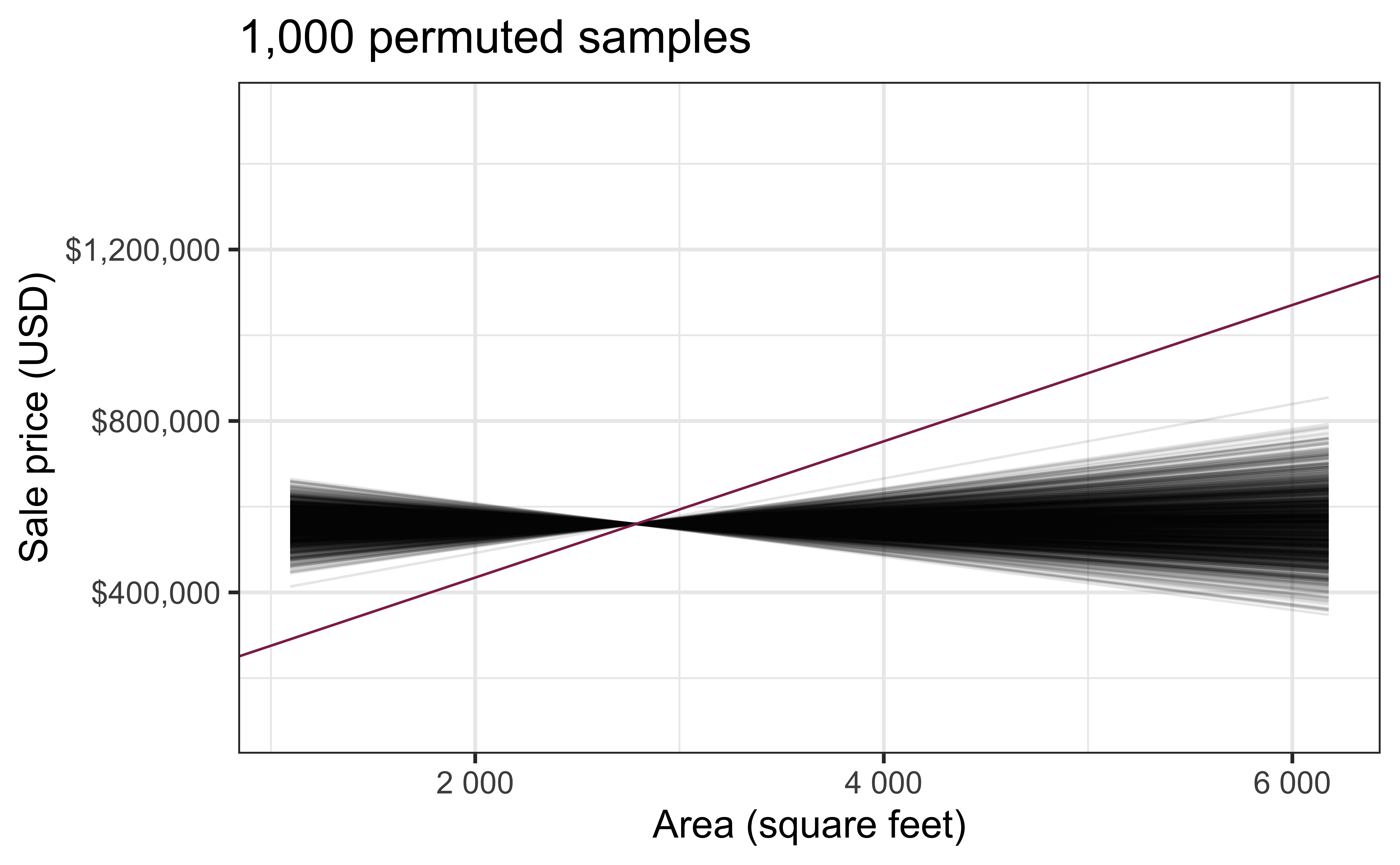
# ℹ 88 more rowsPermutation, visualized
- Each of the observed values for
area(and forprice) exist in both the observed data plot as well as the permutedpriceplot - The permutation removes the relationship between
areaandprice
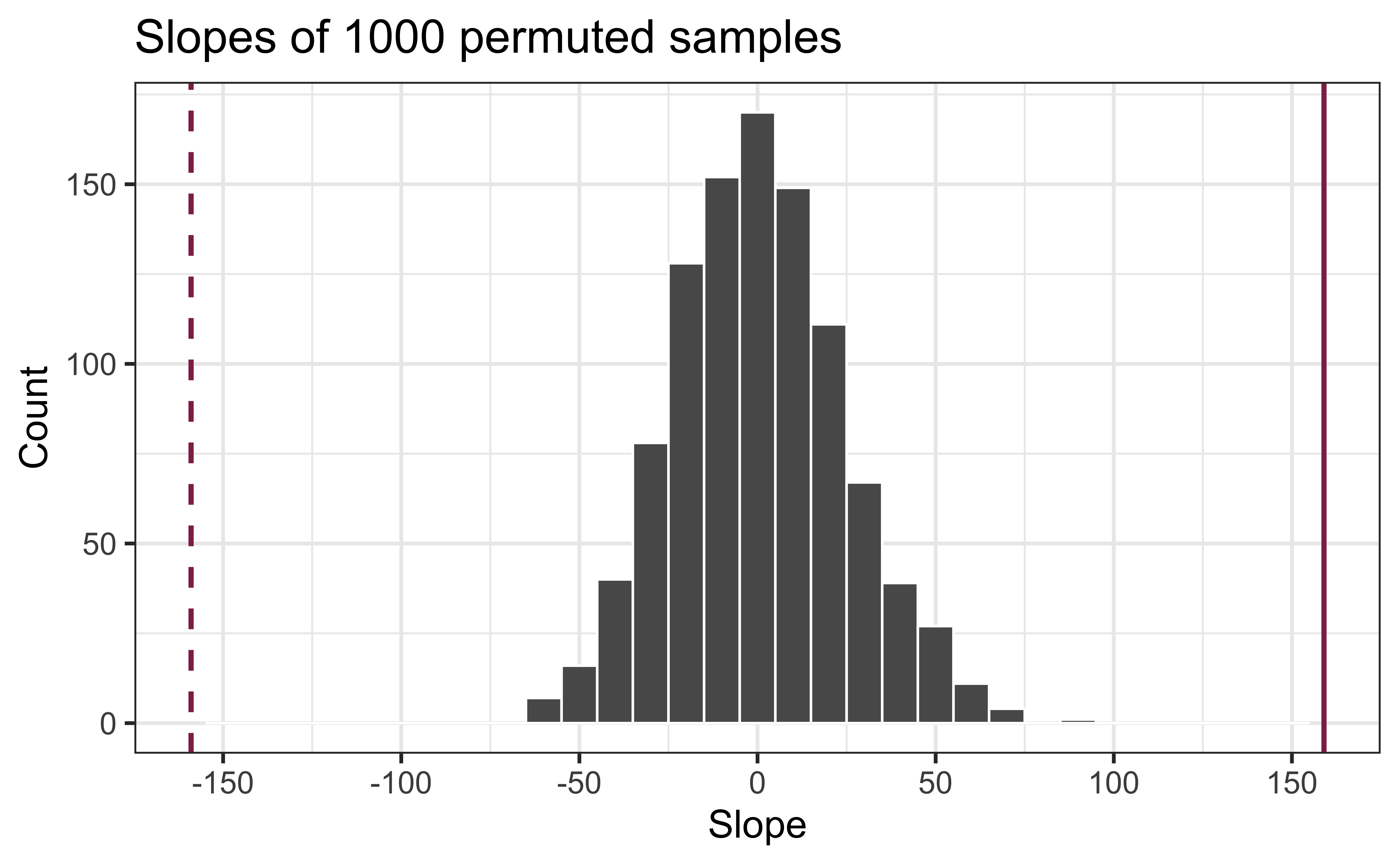
Permutation, repeated
Repeated permutations allow for quantifying the variability in the slope under the condition that there is no linear relationship (i.e., that the null hypothesis is true)
Concluding the hypothesis test
Is the observed slope of \(\hat{\beta_1} = 159\) (or an even more extreme slope) a likely outcome under the null hypothesis that \(\beta = 0\)? What does this mean for our original question: “Do the data provide sufficient evidence that \(\beta_1\) (the true slope for the population) is different from 0?”
Permutation pipeline I
Response: price (numeric)
Explanatory: area (numeric)
# A tibble: 98 × 2
     price  area
     <dbl> <dbl>
 1 1520000  6040
 2 1030000  4475
 3  420000  1745
 4  680000  2091
 5  428500  1772
 6  456000  1950
 7 1270000  3909
 8  557450  2841
 9  697500  3924
10  650000  2173
# ℹ 88 more rowsPermutation pipeline II
Response: price (numeric)
Explanatory: area (numeric)
Null Hypothesis: independence
# A tibble: 98 × 2
price area
<dbl> <dbl>
1 1520000 6040
2 1030000 4475
3 420000 1745
4 680000 2091
5 428500 1772
6 456000 1950
7 1270000 3909
8 557450 2841
9 697500 3924
10 650000 2173
# ℹ 88 more rowsPermutation pipeline III
set.seed(1125)

duke_forest |>
specify(price ~ area) |>
hypothesize(null = "independence") |>
generate(reps = 1000, type = "permute")Response: price (numeric)
Explanatory: area (numeric)
Null Hypothesis: independence
# A tibble: 98,000 × 3
# Groups: replicate [1,000]
price area replicate
<dbl> <dbl> <int>
1 465000 6040 1
2 481000 4475 1
3 1020000 1745 1
4 520000 2091 1
5 592000 1772 1
6 650000 1950 1
7 473000 3909 1
8 705000 2841 1
9 785000 3924 1
10 671500 2173 1
# ℹ 97,990 more rowsPermutation pipeline IV
set.seed(1125)

duke_forest |>
  specify(price ~ area) |>
hypothesize(null = "independence") |>
generate(reps = 1000, type = "permute") |>
fit()# A tibble: 2,000 × 3
# Groups: replicate [1,000]
replicate term estimate
<int> <chr> <dbl>
1 1 intercept 553355.
2 1 area 2.35
3 2 intercept 635824.
4 2 area -27.3
5 3 intercept 536072.
6 3 area 8.57
7 4 intercept 598649.
8 4 area -13.9
9 5 intercept 556202.
10 5 area 1.33
# ℹ 1,990 more rowsPermutation pipeline V
Visualize the null distribution
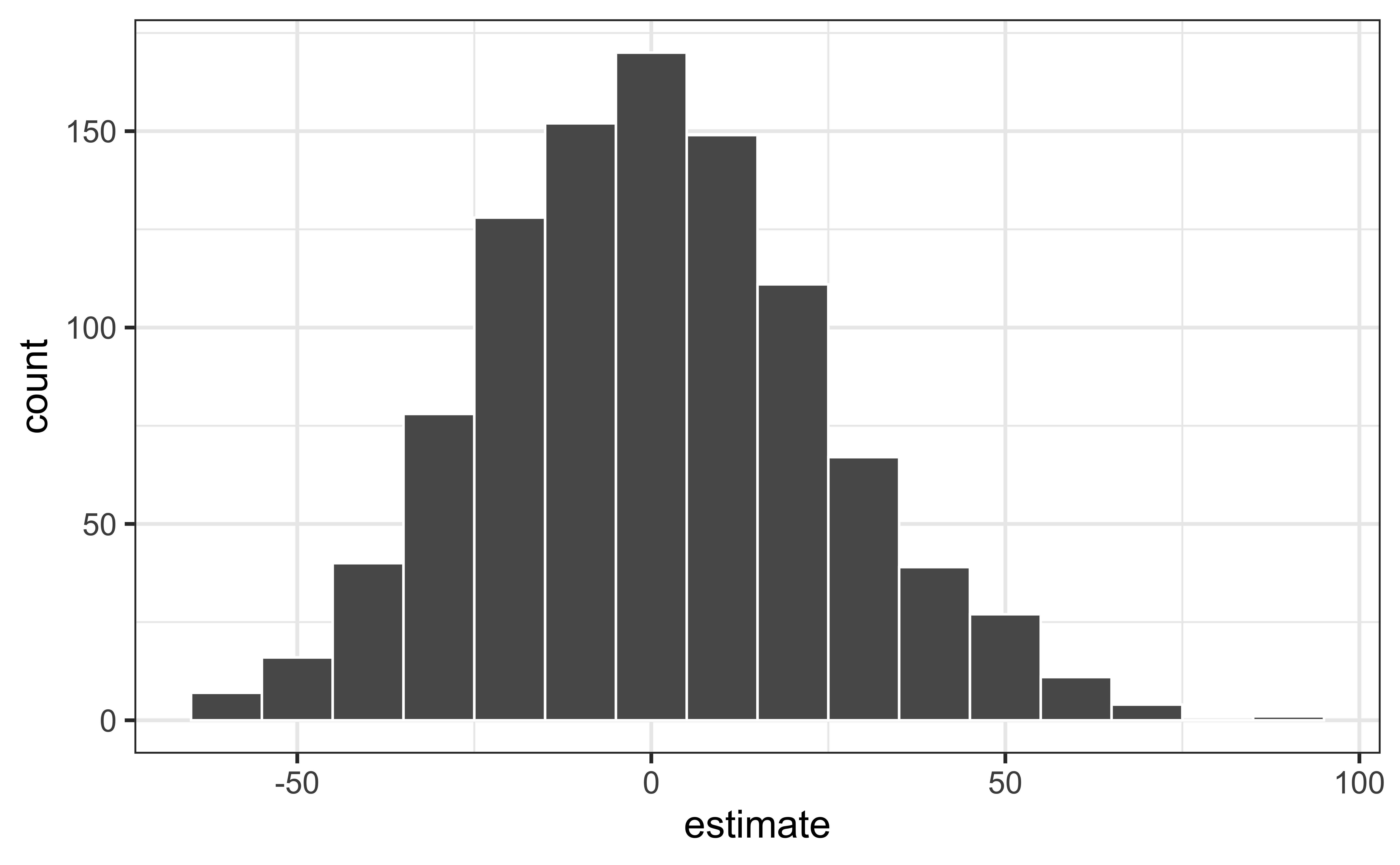
Reason around the p-value
In a world where the there is no relationship between the area of a Duke Forest house and in its price (\(\beta_1 = 0\)), what is the probability that we observe a sample of 98 houses where the slope fo the model predicting price from area is 159 or even more extreme?
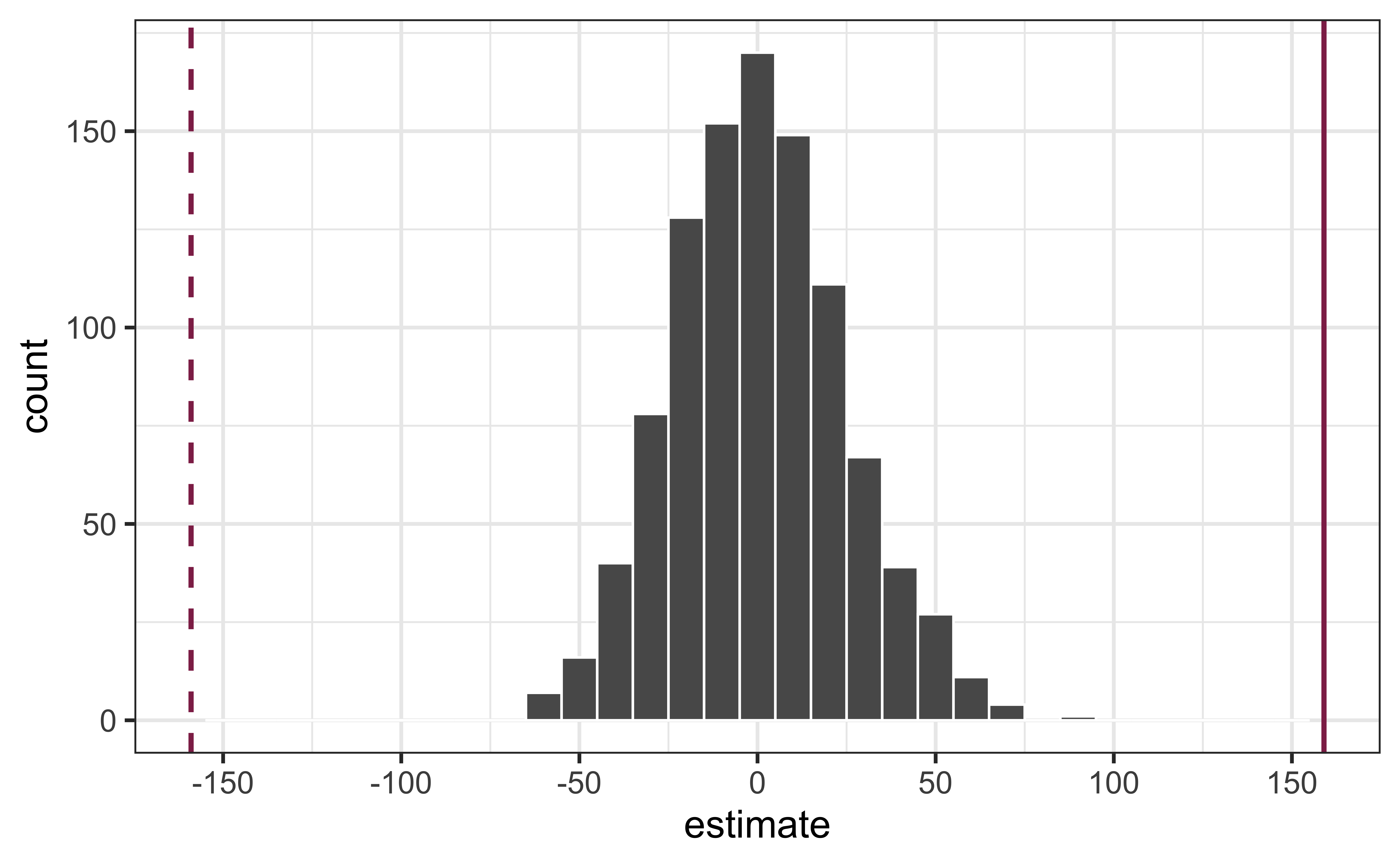
Compute the p-value
What does this warning mean?
get_p_value(
  null_dist,
  obs_stat = obs_fit,
  direction = "two-sided"
)
Warning: Please be cautious in reporting a p-value of 0. This result is an approximation
based on the number of `reps` chosen in the `generate()` step.
ℹ See `get_p_value()` (`?infer::get_p_value()`) for more information.
Please be cautious in reporting a p-value of 0. This result is an approximation
based on the number of `reps` chosen in the `generate()` step.
ℹ See `get_p_value()` (`?infer::get_p_value()`) for more information.# A tibble: 2 × 2
term p_value
<chr> <dbl>
1 area 0
2 intercept 0Application exercise
Mathematical models for inference
The regression model, revisited
df_fit <- lm(price ~ area, data = duke_forest)

tidy(df_fit) |>
kable(digits = 3)| term | estimate | std.error | statistic | p.value |
|---|---|---|---|---|
| (Intercept) | 116652.325 | 53302.463 | 2.188 | 0.031 |
| area | 159.483 | 18.171 | 8.777 | 0.000 |
Inference, revisited
- Earlier we computed a confidence interval and conducted a hypothesis test via simulation:
- CI: Bootstrap the observed sample to simulate the distribution of the slope
- HT: Permute the observed sample to simulate the distribution of the slope under the assumption that the null hypothesis is true
- Now we’ll do these based on theoretical results, i.e., by using the Central Limit Theorem to define the distribution of the slope and use features (shape, center, spread) of this distribution to compute bounds of the confidence interval and the p-value for the hypothesis test
Mathematical representation of the model
\[ \begin{aligned} Y &= \text{Model} + \text{Error} \\ &= f(X) + \epsilon \\ &= \mu_{Y|X} + \epsilon \\ &= \beta_0 + \beta_1 X + \epsilon \end{aligned} \]
where the errors are independent and normally distributed (now we are making an assumption about the distribution of the error terms)
. . .
- independent: Knowing the error term for one observation doesn’t tell you anything about the error term for another observation
- normally distributed: \(\epsilon \sim N(0, \sigma_\epsilon^2)\)
Simple linear regression model fully specified
\[ \mathbf{Y} = \beta_0 + \beta_1X + \epsilon, \quad \epsilon \sim N(0, \sigma^2_{\epsilon}) \]
\(\beta_0\): the population intercept
\(\beta_1\): the population slope
\(\epsilon\) : independent and identically distributed (i.i.d.) error terms
Mathematical representation, visualized
\[ Y|X \sim N(\beta_0 + \beta_1 X, \sigma_\epsilon^2) \]
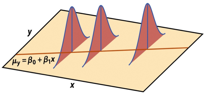
- Mean: \(\beta_0 + \beta_1 X\), the expected value of \(Y\) based on the regression model
- Variance: \(\sigma_\epsilon^2\), constant across the range of \(X\)
- How do we estimate \(\sigma_\epsilon^2\)?
Regression standard error
Once we fit the model, we can use the residuals to estimate the regression standard error (the spread of the distribution of the response, for a given value of the predictor variable):
\[ \hat{\sigma}_\epsilon = \sqrt{\frac{\sum_\limits{i=1}^n(y_i - \hat{y}_i)^2}{n-2}} = \sqrt{\frac{\sum_\limits{i=1}^ne_i^2}{n-2}} \]
. . .
- Why divide by \(n - 2\)?
- Why do we care about the value of the regression standard error?
Standard error of \(\hat{\beta}_1\)
\[ SE_{\hat{\beta}_1} = \hat{\sigma}_\epsilon\sqrt{\frac{1}{(n-1)s_X^2}} \]
. . .
or…
| term | estimate | std.error | statistic | p.value |
|---|---|---|---|---|
| (Intercept) | 116652.33 | 53302.46 | 2.19 | 0.03 |
| area | 159.48 | 18.17 | 8.78 | 0.00 |