library(tidyverse)  # for data wrangling
library(tidymodels) # for modeling and inference
library(knitr)      # to neatly format tables
library(patchwork)  # to arrange plots in a grid

# load other packages as needed HW 02: Multiple linear regression
Important
This assignment is due on Tuesday, February 11 at 11:59pm. To be considered on time, the following must be done by the due date:
Final
.qmdand.pdffiles pushed to your GitHub repoFinal
.pdffile submitted on Gradescope
Introduction
In this analysis you will use multiple linear regression to fit and evaluate models using characteristics of LEGO sets to understand variability in the price.
Learning goals
In this assignment, you will…
- Conduct exploratory data analysis
- Create new variables
- Evaluate and compare models
- Use inference to draw conclusions
- Continue developing a workflow for reproducible data analysis
Getting started
Go to the sta210-sp25 organization on GitHub. Click on the repo with the prefix hw-02. It contains the starter documents you need to complete the lab.
Clone the repo and start a new project in RStudio. See the Lab 00 for details on cloning a repo and starting a new project in R.
The following packages will be used in this assignment:
Data: LEGO sets
The data for this analysis includes information about LEGO sets from themes produced January 1, 2018 and September 11, 2020. The data were originally scraped from Brickset.com, an online LEGO set guide and were obtained for this assignment from Peterson and Ziegler (2021).
You will work with data on about 400 randomly selected LEGO sets produced during this time period. The primary variables are interest in this analysis are
Amazon_Price: Amazon price of the set scraped from brickset.com (in U.S. dollars)Size: General size of the interlocking bricks (Large = LEGO Duplo sets - which include large brick pieces safe for children ages 1 to 5, Small = LEGO sets which- include the traditional smaller brick pieces created for age groups 5 and - older, e.g., City, Friends)Theme: Theme of the LEGO setPages: Number of pages in the instruction booklet
legos <- read_csv("data/lego-sample.csv") |>
  select(Size, Theme, Amazon_Price, Pages) |>
drop_na()Exercises1
Important
All narrative should be written in complete sentences, and all visualizations should have informative titles and axis labels.
Exercise 1
There are some observations that have missing data for any of the variables of interest .
- Remove observations that have missing data for any of the variables of interest -
Size,Theme,Pages, andAmazon_Price. Your updated data set will have 374 observations. - What is a disadvantage of dropping observations that have missing values, instead of using a method to impute, i.e., fill in, the missing data? How might dropping these observations impact the generalizability of conclusions?
Exercise 2
- Visualize the distributions of the predictor variables
SizeandPages. Neatly arrange the plots using the patchwork package. - Use the plots in part (a) to write an observation about each distribution.
Exercise 3
The distribution of Theme is shown below. The bars are ordered by the frequency they occur in the data set.
legos |>
  count(Theme) |>
ggplot(aes(x = fct_reorder(Theme, n), y = n)) +
  geom_col() +
    labs(title = "Lego Set Theme",
         x = "Theme",
         y = "Number of LEGO sets") +
  coord_flip()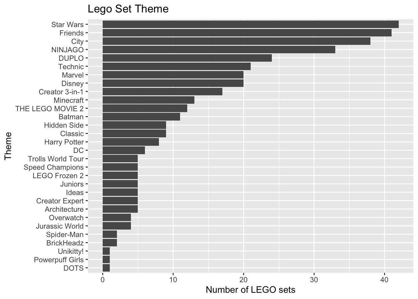
- What is one reason we may want to avoid putting the variable
Themein a model as is? - We will create a new variable that collapses some of the levels of
Theme. Make a new variable calledTheme_Colthat has levels for the top four most frequent themes, then the categoryOtherfor all other themes. - How many observations are in each level for the new variable created in part (b)?
Note
You will use Theme_Col, the collapsed Theme variable, for the remainder of the assignment.
Exercise 4
- Fit a model using
Size,Pages, andTheme_Colto predictAmazon_Price. Fit the model such that the intercept has a meaningful interpretation. Neatly display the model using three digits. - Interpret the intercept in the context of the data.
- The model output suggests that as the number of pages in the instruction booklet increases, the price of the set on Amazon is expected to increase. On the surface, it does not seem that the number of pages in the booklet would be a major predictor of the price on Amazon. What do you think this variable is actually measuring or is actually representing?
Exercise 5
Now let’s consider a model that allows for different effects of pages based on theme.
- Make a plot that can be used to visualize the effect of pages on the Amazon.com price based on the theme.
- Based on the plot in part (a), does the effect of the number of pages appear to differ based on theme? Briefly explain why or why not.
- Modify the model from Exercise 4 such that the effect of the number of pages differs based on the theme. The intercept should still have a meaningful interpretation. Neatly display the model using three digits.
Exercise 6
- Describe the effect of pages for the baseline level in the context of the data.
- Describe the effect of pages for LEGOS in the Star Wars theme in the context of the data.
- Based on the p-values, do the data provide evidence that the effect of pages differs based on theme? Briefly explain. You can use a threshold of 0.05 for your assessment.
Exercise 7
Compute RMSE for the model in Exercise 5. Interpret this value in the context of the data.
Compute \(R^2\) for the model in Exercise 5. Interpret this value in the context of the data.
Perceived threat of COVID-19
Important
Use the following paper for Exercises 8 and 9.
Garbe, Rau, and Toppe (2020) aimed to examine the relationship between personality traits, perceived threat of Covid-19 and stockpiling toilet paper. For this study, researchers conducted an online survey March 23 - 29, 2020 and used the results to fit multiple linear regression models to draw conclusions about their research questions. From their survey, they collected data on adults across 35 countries. Given the small number of responses from people outside of the United States, Canada, and Europe, only responses from people in these three locations were included in the regression analysis.
Let’s consider their results for the model looking at the effect on perceived threat of Covid-19. The model can be found on page 6 of the paper. The perceived threat of Covid was quantified using the responses to the following survey question:
How threatened do you feel by Coronavirus? [Users select on a 10-point visual analogue scale (Not at all threatened to Extremely Threatened)]
As stated on page 5 of the paper “To ease interpretation, continuous variables were z-standardized and categorical variables were dummy-coded in all models.”
Click here to access a PDF of the paper.
Exercise 8
Interpret the coefficient of Age (0.072) in the context of the analysis.
Interpret the coefficient of Place of residence in the context of the analysis. You can assume
Emotionality = 0in the interpretation.The model includes an interaction between Place of residence and Emotionality. The authors describe Emotionality as a measure of “fearfulness, anxiety, dependence, sentimentality”. What does the coefficient for the interaction (0.101) mean in the context of the data?
Important
The following are general questions about linear regression. They are not specific to any of the previous analyses.
Exercise 9
Prove that the maximum value of \(R^2\) must be less than 1 if the data set contains observations such that there are different observed values of the response for the same value of the predictor (e.g., the data set contains observations \((x_i, y_i)\) and \((x_j, y_j)\) such that \(x_i = x_j\) and \(y_i \neq y_j\) .
Exercise 10
In lecture we discussed how the distribution of the error terms (and thus the distribution of the response variable \(Y\)) for a given value of the predictor \(X\) has a variance of \(\sigma^2_{\epsilon}\). Therefore, we are assuming this variance is the same for all values of the predictor when we conduct inference.
Briefly explain why this assumption is important when we conduct inference based on mathematical models but is not necessary for conducting simulation-based inference.
Submission
Warning
Before you wrap up the assignment, make sure all documents are updated on your GitHub repo. We will be checking these to make sure you have been practicing how to commit and push changes.
Remember – you must turn in a PDF file to the Gradescope page before the submission deadline for full credit.
To submit your assignment:
Access Gradescope through the STA 210 Canvas site.
Click on the assignment, and you’ll be prompted to submit it.
Mark the pages associated with each exercise. All of the pages of your lab should be associated with at least one question (i.e., should be “checked”).
Select the first page of your .PDF submission to be associated with the “Workflow & formatting” section.
Grading (50 points)
| Component | Points |
|---|---|
| Ex 1 | 3 |
| Ex 2 | 5 |
| Ex 3 | 4 |
| Ex 4 | 6 |
| Ex 5 | 6 |
| Ex 6 | 6 |
| Ex 7 | 4 |
| Ex 8 | 6 |
| Ex 9 | 4 |
| Ex 10 | 3 |
| Workflow & formatting | 3 |
The “Workflow & formatting” grade is to assess the reproducible workflow and document format for the applied exercises. This includes having at least 3 informative commit messages, a neatly organized document with readable code and your name and the date updated in the YAML.
References
Garbe, Lisa, Richard Rau, and Theo Toppe. 2020. “Influence of Perceived Threat of Covid-19 and HEXACO Personality Traits on Toilet Paper Stockpiling.” Edited by Valerio Capraro. PLOS ONE 15 (6): e0234232. https://doi.org/10.1371/journal.pone.0234232.
Montgomery, Douglas C, Elizabeth A Peck, and G Geoffrey Vining. 2021. Introduction to Linear Regression Analysis. John Wiley & Sons.
Peterson, Anna D., and Laura Ziegler. 2021. “Building a Multiple Linear Regression Model With LEGO Brick Data.” Journal of Statistics and Data Science Education 29 (3): 297–303. https://doi.org/10.1080/26939169.2021.1946450.