# load packages
library(tidyverse)
library(tidymodels)
library(knitr)
library(patchwork)

# set default theme in ggplot2
ggplot2::theme_set(ggplot2::theme_bw())Variable transformations cont’d
Announcements
Lab 04 due TODAY at 11:59pm
HW 03 due Tuesday March 18 at 11:59pm
Next project milestone: Exploratory data analysis due March 20
- Work on it in lab March 17
Computing set up
Topics
- Log-transformation on the predictor
Math rules
\[ \begin{aligned} \log(ab) &= \log(a) + \log(b) \\[8pt] \log\big(\frac{a}{b}\big) &= \log(a) - \log(b)\\[15pt] e^{a + b + c} &= e^ae^be^c \\[8pt] e^{a - b} &= \frac{e^a}{e^b} \end{aligned} \]
Data: Life expectancy in 140 countries
The data set comes from Zarulli et al. (2021) who analyze the effects of a country’s healthcare expenditures and other factors on the country’s life expectancy. The data are originally from the Human Development Database and World Health Organization.
There are 140 countries (observations) in the data set.
Click here for the original research paper.
Variables
life_exp: The average number of years that a newborn could expect to live, if he or she were to pass through life exposed to the sex- and age-specific death rates prevailing at the time of his or her birth, for a specific year, in a given country, territory, or geographic income_inequality. ( from the World Health Organization)income_inequality: Measure of the deviation of the distribution of income among individuals or households within a country from a perfectly equal distribution. A value of 0 represents absolute equality, a value of 100 absolute inequality (based on Gini coefficient). (from Zarulli et al. (2021))
Variables
education: Indicator of whether a country’s education index is above (High) or below (Low) the median index for the 140 countries in the data set.- Education index: Average of mean years of schooling (of adults) and expected years of school (of children), both expressed as an index obtained by scaling wit the corresponding maxima.
health_expend: Per capita current spending on on healthcare goods and services, expressed in respective currency - international Purchasing Power Parity (PPP) dollar (from the World Health Organization)
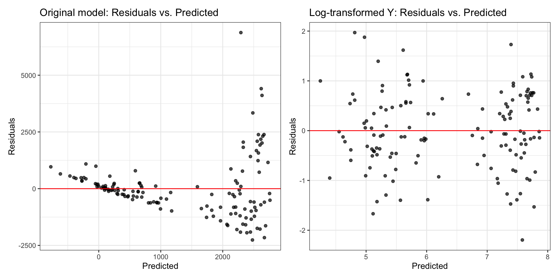
Review: Model with log(Y)
| term | estimate | std.error | statistic | p.value |
|---|---|---|---|---|
| (Intercept) | 7.096 | 0.324 | 21.895 | 0 |
| income_inequality | -0.065 | 0.011 | -5.714 | 0 |
| educationHigh | 1.117 | 0.218 | 5.121 | 0 |
For each additional point in the income inequality index, a country’s health expenditures are expected to multiply by 0.937 \((e^{-0.065})\), holding education constant.
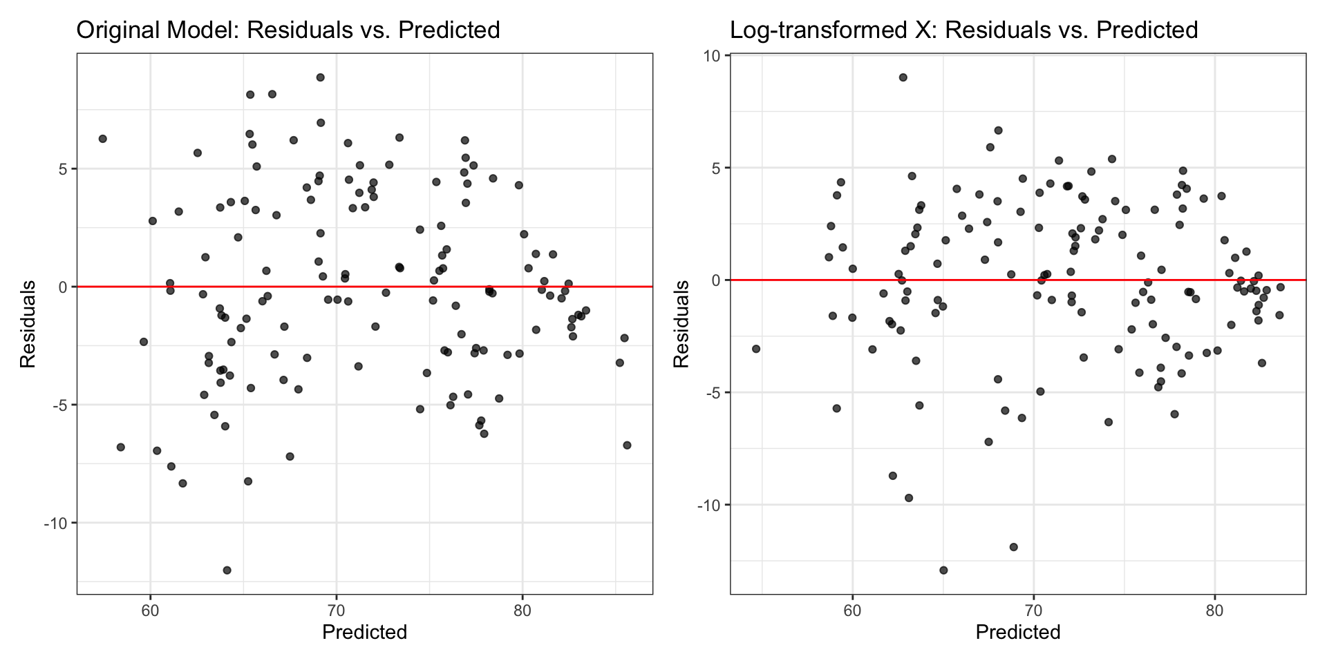
Compare residual plots
Log transformation on a predictor variable
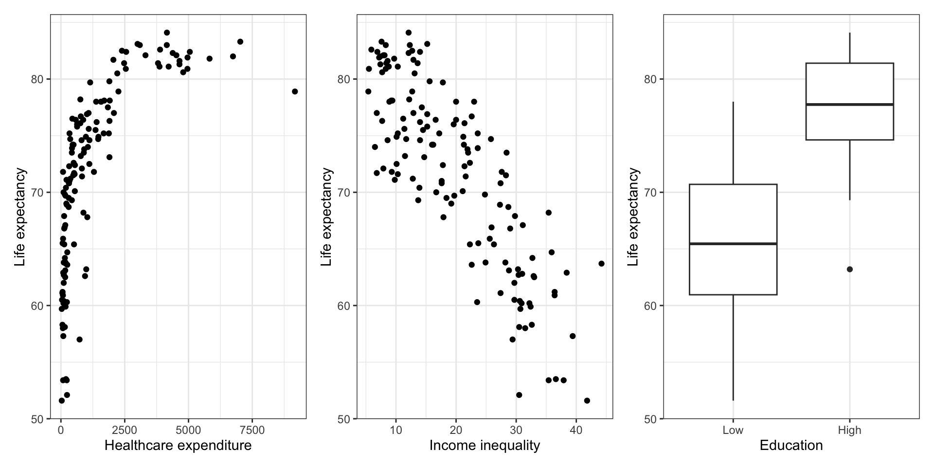
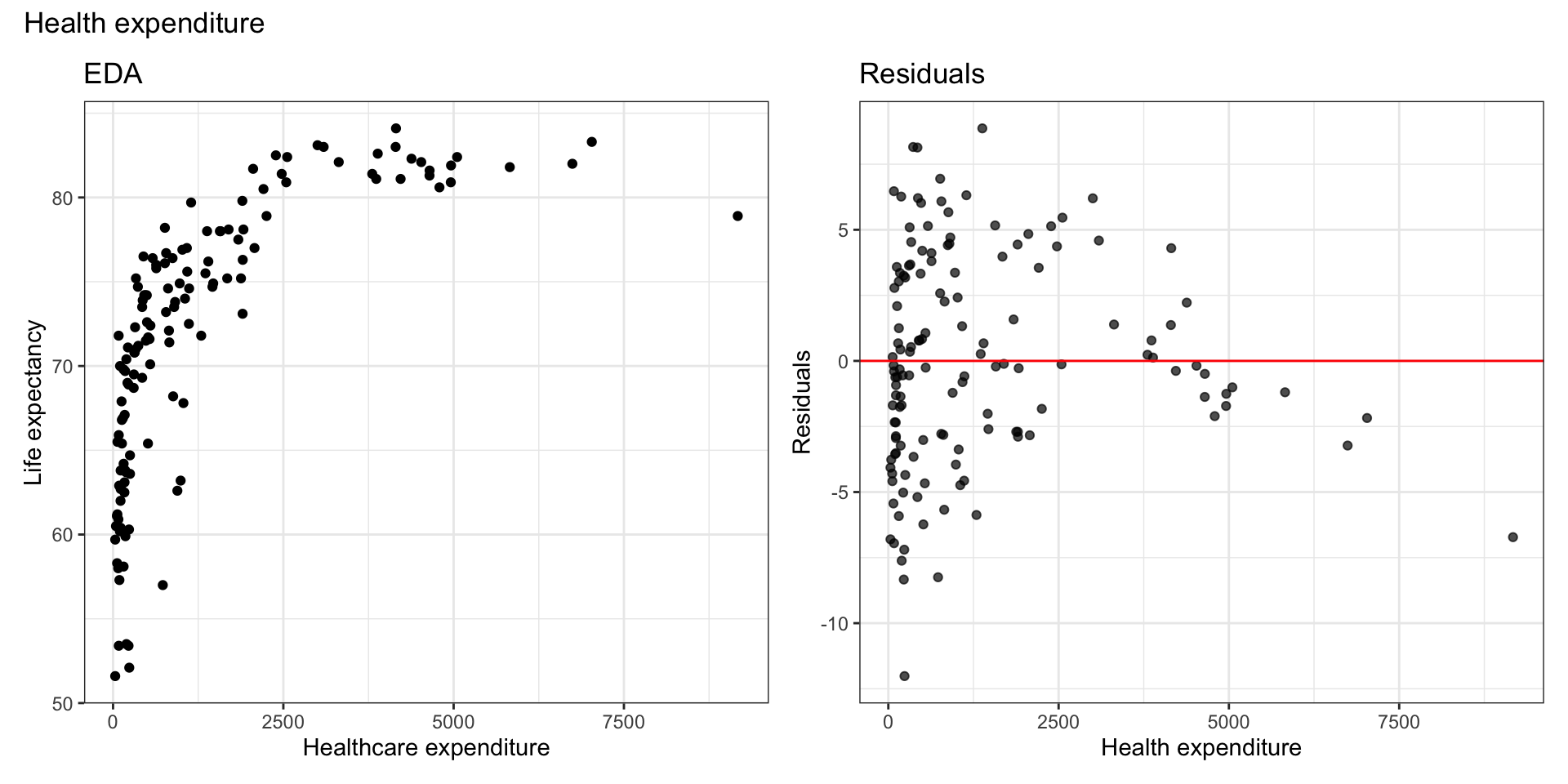
Variability in life expectancy
Let’s consider a model using a country’s healthcare expenditure, income inequality, and education to predict its life expectancy
Original model
life_exp_fit <- lm(life_exp ~ health_expenditure + income_inequality + education,
data = health_data)| term | estimate | std.error | statistic | p.value |
|---|---|---|---|---|
| (Intercept) | 78.575 | 1.775 | 44.274 | 0.000 |
| health_expenditure | 0.001 | 0.000 | 4.522 | 0.000 |
| income_inequality | -0.484 | 0.061 | -7.900 | 0.000 |
| educationHigh | 2.020 | 1.168 | 1.730 | 0.086 |
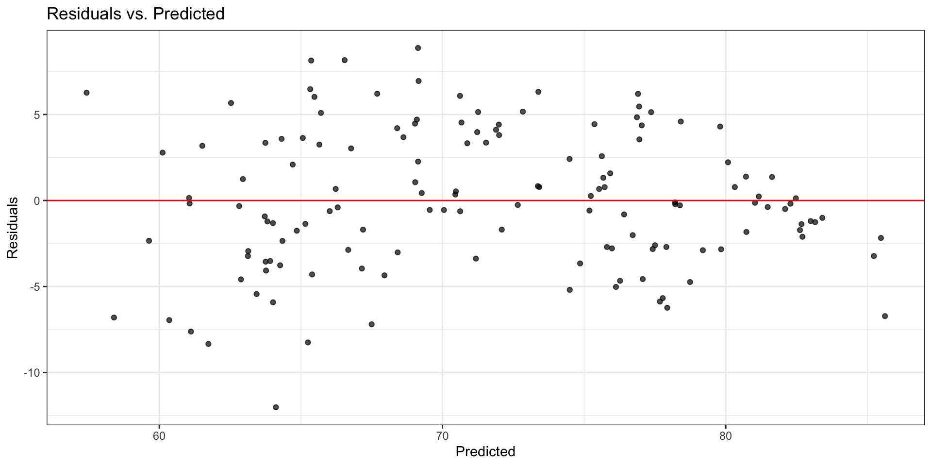
Original model: Residuals
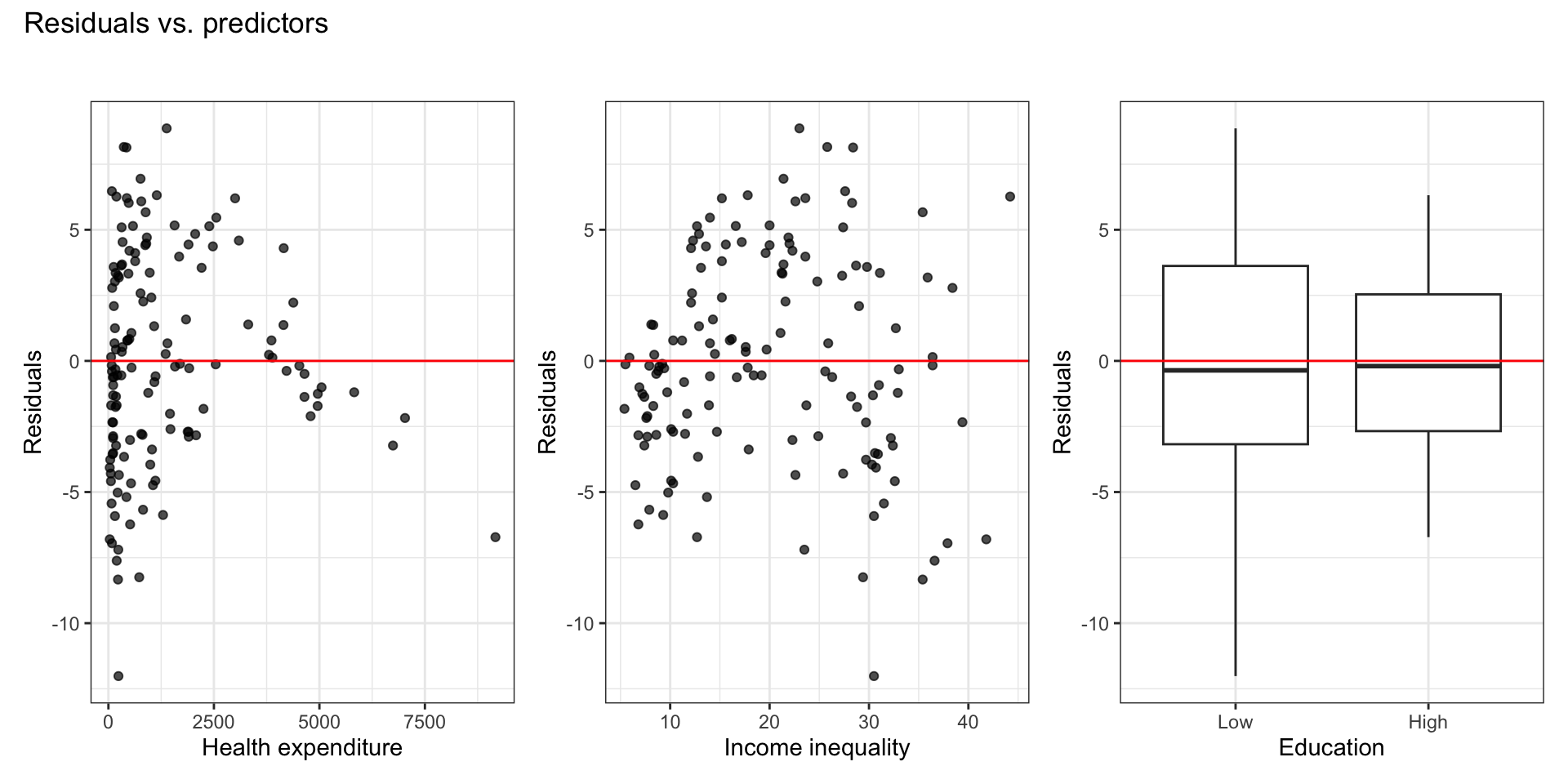
Residuals vs. predictors
. . .
There is a non-linear relationship is between health expenditure and life expectancy.
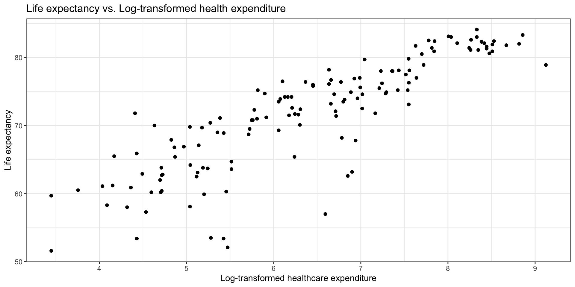
Log Transformation on \(X\)
Try a transformation on \(X\) if the scatterplot in EDA shows non-linear relationship and residuals vs. fitted looks parabolic
EDA
Model with Transformation on \(X_j\)
When we fit a model with predictor \(\log(X_j)\), we fit a model of the form
\[ Y = \beta_0 + \beta_1X_1 + \dots + \beta_j\log(X_j) + \dots \beta_pX_p + \epsilon, \quad \epsilon \sim N(0, \sigma^2_{\epsilon}) \]
The estimated regression model is
\[ \hat{y}_i = \hat{\beta}_0 + \hat{\beta}_1x_{i1} + \ldots + \hat{\beta}_j\log(x_{ij}) + \dots + \hat{\beta}_px_{ip} \]
Model interpretation
\[ \hat{y}_i = \hat{\beta}_0 + \hat{\beta}_1x_{i1} + \ldots + \hat{\beta}_j\log(x_{ij}) + \dots + \hat{\beta}_px_{ip} \]
Intercept: When \(x_{i1} = \dots = \log(x_{ij}) = \dots = x_{ip} = 0\) , \(y_i\) is expected to be \(\hat{\beta}_0\), on average.
- \(\log(x_{ij}) = 0\) when \(x_{ij} = 1\)
Coefficient of \(X_j\): When \(x_{ij}\) is multiplied by a factor of \(C\), \(y_i\) is expected to change by \(\hat{\beta}_j\log(C)\) units, on average, holding all else constant.
- Example: When \(x_{ij}\) is multiplied by a factor of 2, \(y_i\) is expected to increase by \(\hat{\beta}_j\log(2)\) units, on average, holding all else constant.
Model with log(X)
life_exp_logx_fit <- lm(life_exp ~ log(health_expenditure) + income_inequality
+ education, data = health_data)| term | estimate | std.error | statistic | p.value |
|---|---|---|---|---|
| (Intercept) | 59.151 | 3.184 | 18.576 | 0.000 |
| log(health_expenditure) | 3.092 | 0.396 | 7.814 | 0.000 |
| income_inequality | -0.362 | 0.058 | -6.225 | 0.000 |
| educationHigh | -0.168 | 1.103 | -0.152 | 0.879 |
Interpret the intercept in the context of the data.
Interpret the effect of health expenditure in the context of the data.
Interpret the effect of education in the context of the data.
Model with log(X): Residuals
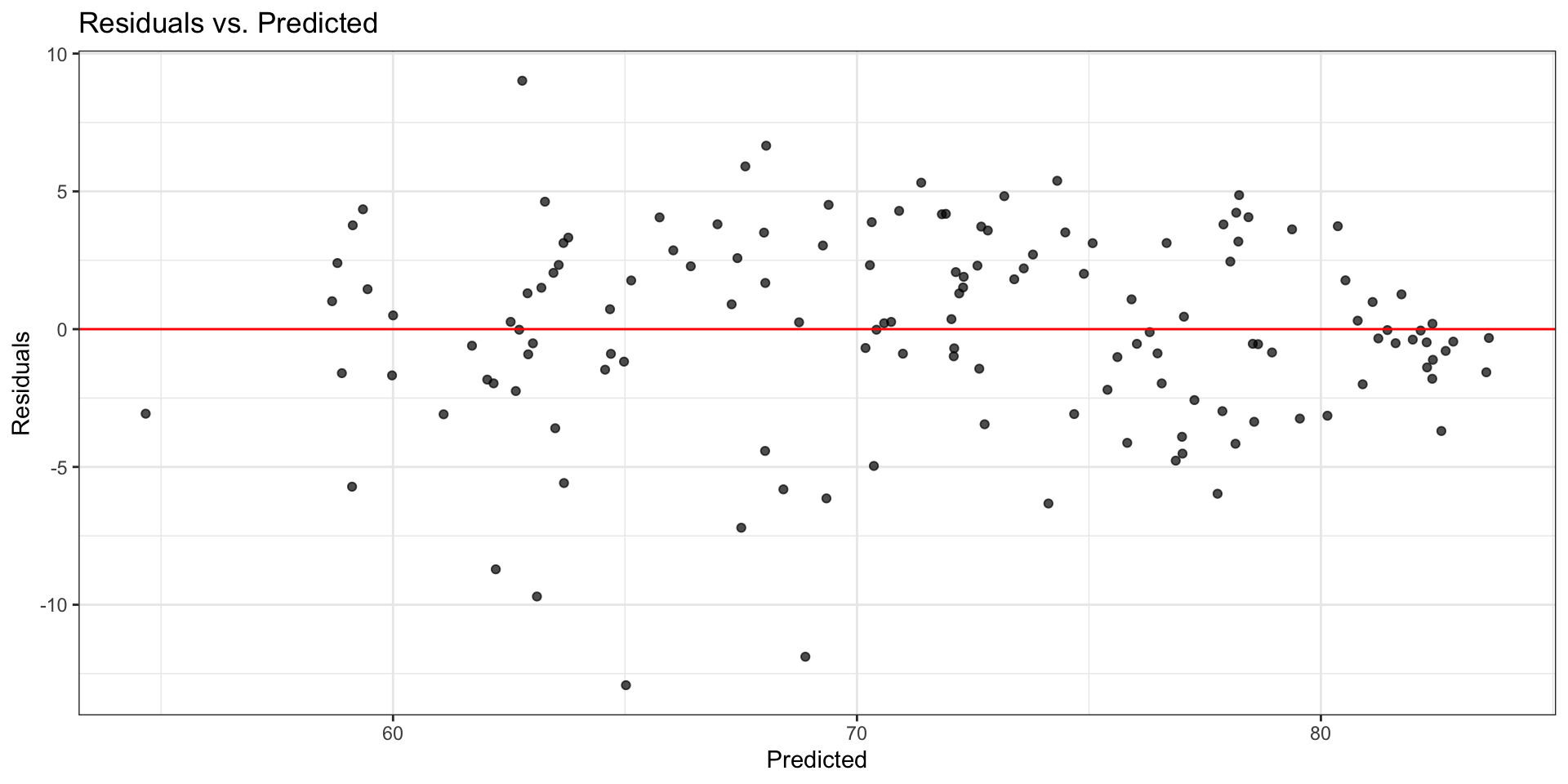
Comparing residual plots
Learn more
See Log Transformations in Linear Regression for more details about interpreting regression models with log-transformed variables.
Recap
- Introduced log-transformation on the predictor
- Identified linear models
References
Zarulli, Virginia, Elizaveta Sopina, Veronica Toffolutti, and Adam Lenart. 2021. “Health Care System Efficiency and Life Expectancy: A 140-Country Study.” Edited by Srinivas Goli. PLOS ONE 16 (7): e0253450. https://doi.org/10.1371/journal.pone.0253450.