AE 03: Simple linear regression

Bike rentals in Washington, DC

Important

Go to the course GitHub organization and locate your ae-03 repo to get started. If you do not see an ae-03 repo, use the link below to create one:

https://classroom.github.com/a/jxxCTVVo

This AE does not count towards the participation grade.

library(tidyverse)
library(tidymodels)
library(patchwork)

Data

Our data set contains daily rentals from the Capital Bikeshare in Washington, DC in 2011 and 2012. It was obtained from the dcbikeshare data set in the dsbox R package.

We will focus on the following variables in the analysis:

• count: total bike rentals
• temp_orig: Temperature in degrees Celsius
• season: 1 - Winter, 2 - Spring, 3 - Summer, 4 - Fall

Click here for the full list of variables and definitions.

bikeshare <- read_csv("data/dcbikeshare.csv")

Exercises

Exercise 1

Visualizations for the univariate and bivariate exploratory data analysis of daily bike rentals and temperature are below.

p1 <- ggplot(bikeshare, aes(x = count)) +
  geom_histogram(binwidth = 250) + 
  labs(x = "Daily bike rentals")

p2 <- ggplot(bikeshare, aes(x = temp_orig)) +
  geom_histogram() + 
  labs(x = "Temperature (Celsius)")

p3 <- ggplot(bikeshare, aes(y = count, x = temp_orig)) +
  geom_point() + 
  labs(x = "Temperature (Celsius)", 
       y = "Daily bike rentals")

(p1 | p2) / p3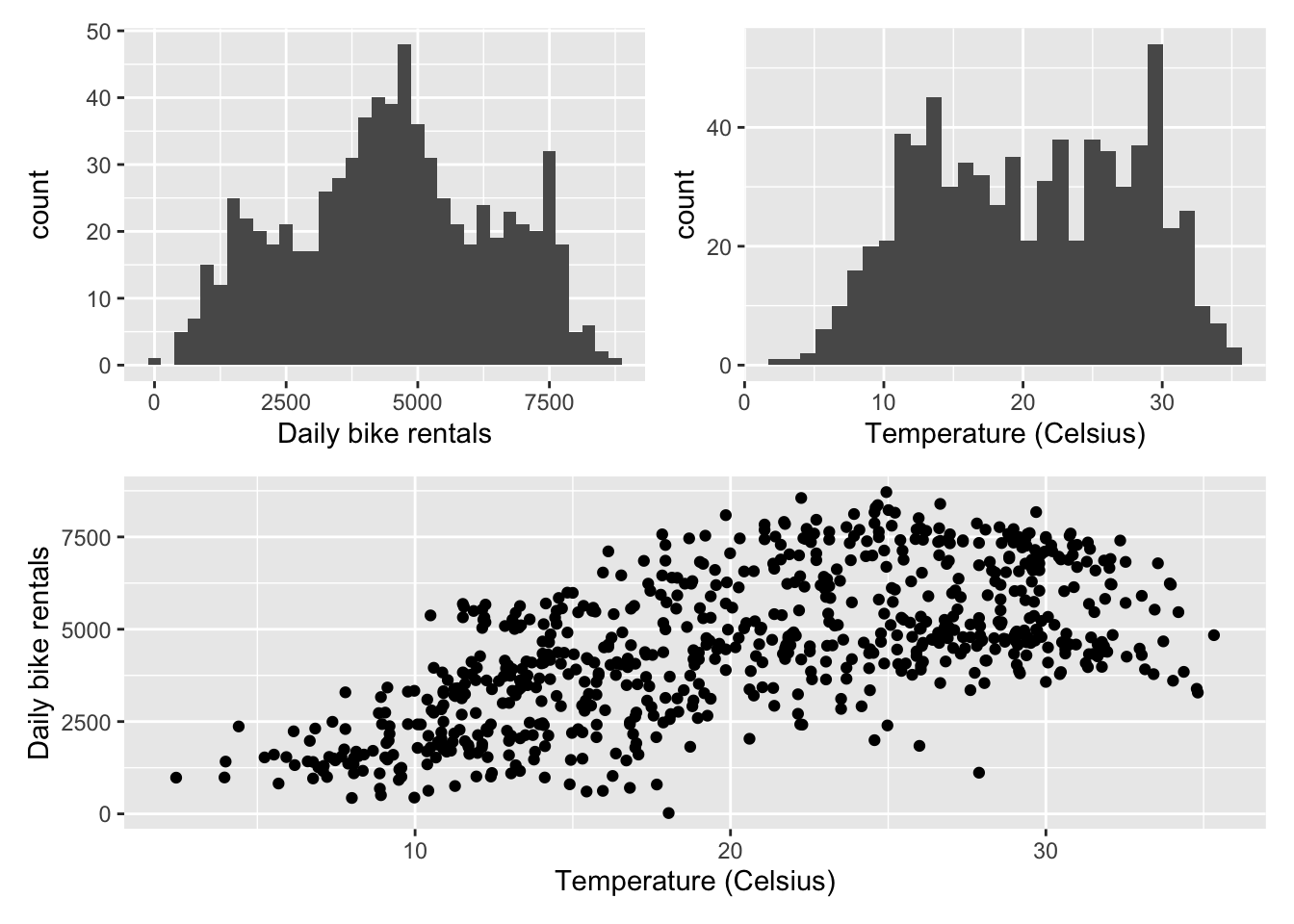

There appears to be one day with a very small number of bike rentals. What was the day? Why were the number of bike rentals so low on that day? Hint: You can Google the date to figure out what was going on that day.

Exercise 2

In the raw data, seasons are coded as 1, 2, 3, 4, numeric values that correspond to winter, spring, summer, and fall respectively. Complete the code below to make season a categorical variable with levels corresponding to season names stored in the original order.

bikeshare <- bikeshare |>
  mutate(season = case_when(
    season == 1 ~ "Winter", 
    season == 2 ~ "Spring", 
    season == 3 ~ "Summer", 
    season == 4 ~ "Fall"
  ))

Exercise 3

We want to evaluate whether the relationship between temperature and daily bike rentals is the same for each season. To answer this question, begin by creating a scatter plot of daily bike rentals vs. temperature faceted by season.

# add code developed during livecoding here

Exercise 4

• Which season appears to have the strongest relationship between temperature and daily bike rentals? Why do you think the relationship is strongest in this season?

• Which season appears to have the weakest relationship between temperature and daily bike rentals? Why do you think the relationship is weakest in this season?

Exercise 5

Filter your data for the season with the strongest apparent relationship between temperature and daily bike rentals.

# add code developed during livecoding here

Exercise 6

Using the data from Exercise 5, fit a linear model to predict daily bike rentals using temperature for this season.

# add code developed during livecoding here

Exercise 7

Use the output to write out the estimated regression equation.

Exercise 8

• Interpret the slope in the context of the data.

• Does it make sense to interpret the intercept? If so, interpret the intercept in the context of the data. Otherwise, explain why not.

Exercise 9

Suppose you work for a bike share company in Durham, NC, and they want to predict daily bike rentals in 2024. What is one reason you might recommend they use your analysis for this task? What is one reason you would recommend they not use your analysis for this task?

Submission

Important

To submit the AE:

• Render the document to produce the PDF with all of your work from today’s class.
• Push all your work to your ae-03- repo on GitHub. (AEs are not submitted on Gradescope.)