Multiple linear regression (MLR)

Prof. Maria Tackett

Jan 30, 2025

Announcements

Lab 01 due TODAY at 11:59pm
Team labs start on Monday
Click here to learn more about the Academic Resource Center
Statistics experience due Tuesday, April 15

Computational setup

# load packages
library(tidyverse)
library(tidymodels)
library(openintro)
library(patchwork)
library(knitr)
library(kableExtra)
library(colorblindr)
library(palmerpenguins)

# set default theme and larger font size for ggplot2
ggplot2::theme_set(ggplot2::theme_minimal(base_size = 16))

Considering multiple variables

Data: Palmer penguins

The penguins data set contains data for penguins found on three islands in the Palmer Archipelago, Antarctica. Data were collected and made available by Dr. Kristen Gorman and the Palmer Station, Antarctica LTER, a member of the Long Term Ecological Research Network. These data can be found in the palmerpenguins R package.

# A tibble: 342 × 4
   body_mass_g flipper_length_mm bill_length_mm species
         <int>             <int>          <dbl> <fct>  
 1        3750               181           39.1 Adelie 
 2        3800               186           39.5 Adelie 
 3        3250               195           40.3 Adelie 
 4        3450               193           36.7 Adelie 
 5        3650               190           39.3 Adelie 
 6        3625               181           38.9 Adelie 
 7        4675               195           39.2 Adelie 
 8        3475               193           34.1 Adelie 
 9        4250               190           42   Adelie 
10        3300               186           37.8 Adelie 
# ℹ 332 more rows

Variables

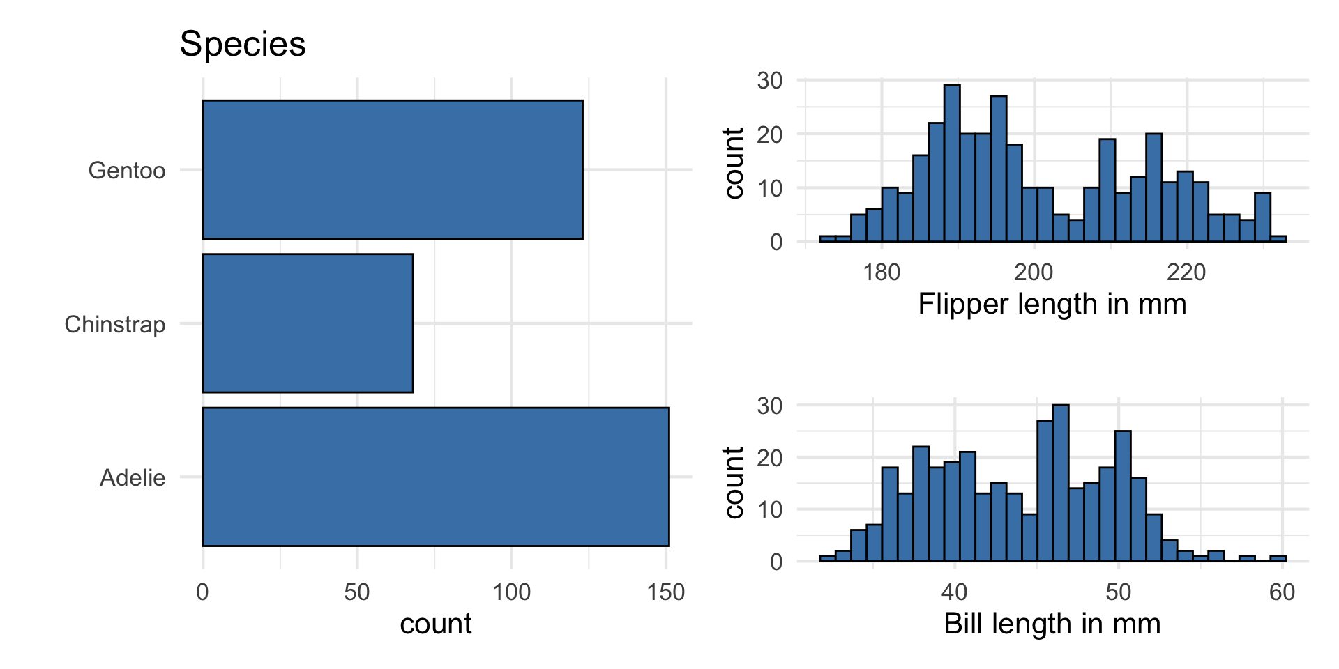
Predictors:

bill_length_mm: Bill length in millimeters
flipper_length_mm: Flipper length in millimeters
species: Adelie, Gentoo, or Chinstrap species

Response: body_mass_g: Body mass in grams

The goal of this analysis is to use the bill length, flipper length, and species to predict body mass.

Response: `body_mass_g`

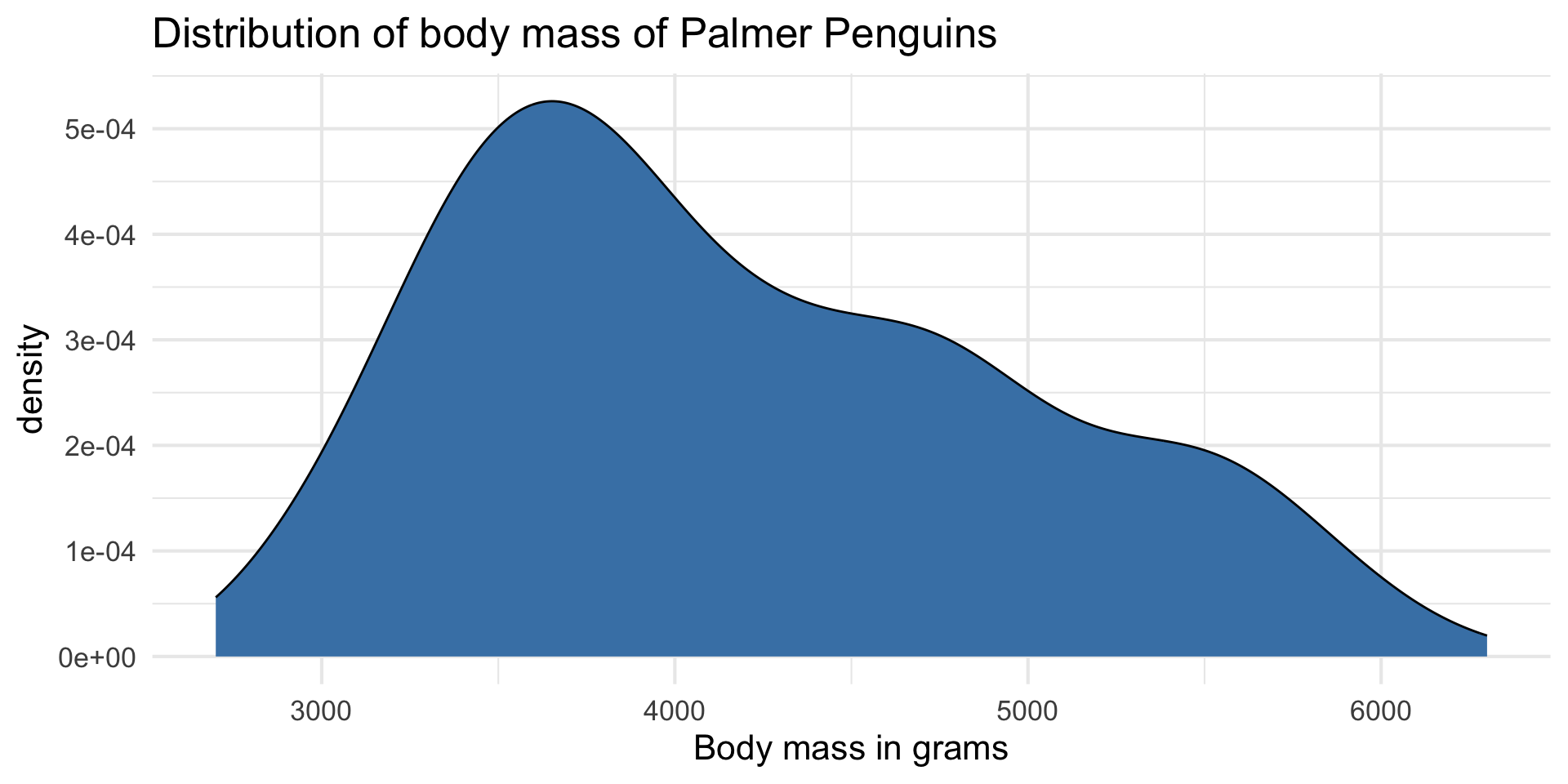
min	median	max	iqr
2700	4050	6300	1200

Predictors

Response vs. predictors

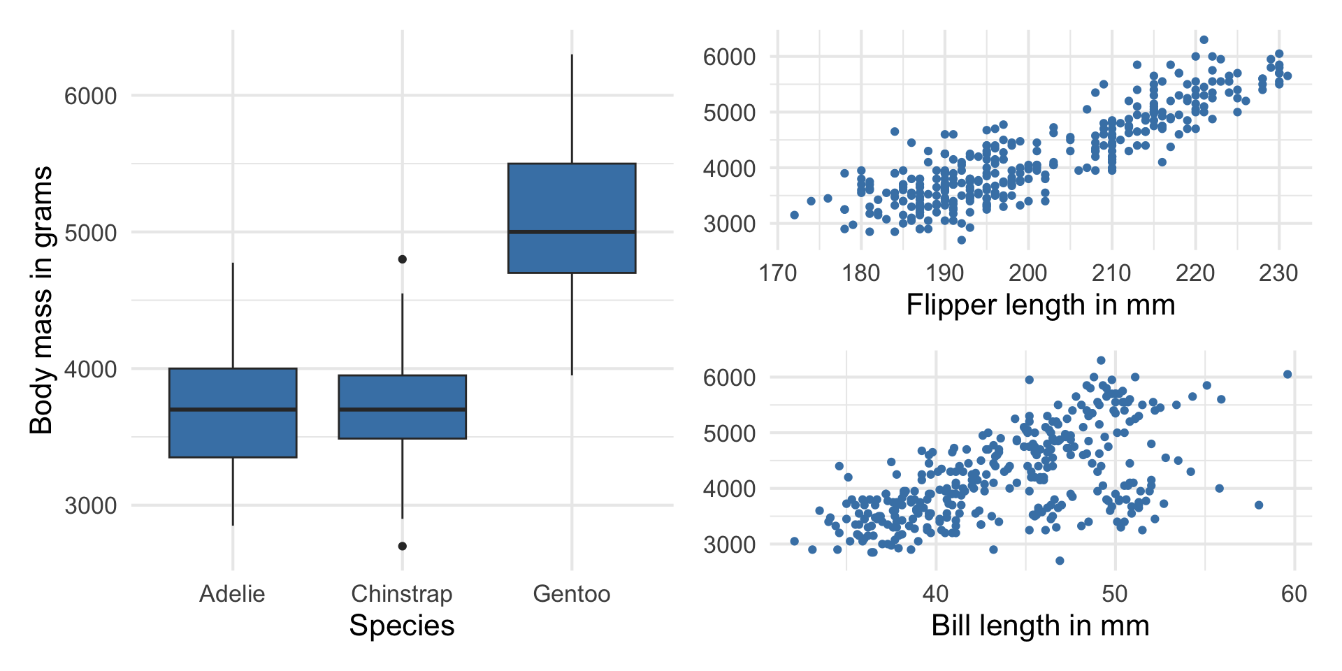
Why do we want to use a single model with all the predictors instead of 3 separate models?

Multiple linear regression

Multiple linear regression (MLR)

Based on the analysis goals, we will use a multiple linear regression model of the following form

\[ \begin{aligned}\widehat{\text{body_mass_g}} ~ = \hat{\beta}_0 & + \hat{\beta}_1 \times \text{flipper_length_mm} \\ & + \hat{\beta}_2 \times \text{species}_1 \\ &+\hat{\beta}_3 \times \text{species}_2 \\ &+ \hat{\beta}_4 \times \text{bill_length_mm} \end{aligned} \]

Similar to simple linear regression, this model assumes that at each combination of the predictor variables, the values body_mass_g follow a Normal distribution.

Multiple linear regression

Recall: The simple linear regression model assumes

\[ Y|X\sim N(\beta_0 + \beta_1 X, \sigma_{\epsilon}^2) \]

Similarly: The multiple linear regression model assumes

\[ Y|X_1, X_2, \ldots, X_p \sim N(\beta_0 + \beta_1 X_1 + \beta_2 X_2 + \dots + \beta_p X_p, \sigma_{\epsilon}^2) \]

Multiple linear regression

At any combination of the predictors, the mean value of the response \(Y\), is

\[ E(Y|X_1, \ldots, X_p) = \beta_0 + \beta_1 X_{1} + \beta_2 X_2 + \dots + \beta_p X_p \]

Using multiple linear regression, we can estimate the mean response for any combination of predictors

\[ \hat{Y} = \hat{\beta}_0 + \hat{\beta}_1 X_{1} + \hat{\beta}_2 X_2 + \dots + \hat{\beta}_p X_{p} \]

Model fit

penguin_fit <- lm(body_mass_g ~ flipper_length_mm + species + 
                bill_length_mm, data = penguins)

tidy(penguin_fit) |>
  kable(digits = 3)

term	estimate	std.error	statistic	p.value
(Intercept)	-3904.387	529.257	-7.377	0.000
flipper_length_mm	27.429	3.176	8.638	0.000
speciesChinstrap	-748.562	81.534	-9.181	0.000
speciesGentoo	90.435	88.647	1.020	0.308
bill_length_mm	61.736	7.126	8.664	0.000

Model equation

\[ \begin{align}\widehat{\text{body_mass_g}} = -3904.387 &+27.429 \times \text{flipper_length_mm}\\ & -748.562 \times \text{Chinstrap}\\ &+ 90.435 \times \text{Gentoo}\\ &+ 61.736 \times \text{bill_length_mm} \end{align} \]

Note

We will talk about why there are two terms in the model for species shortly!

Interpreting \(\hat{\beta}_j\)

The estimated coefficient \(\hat{\beta}_j\) is the expected change in the mean of \(Y\) when \(X_j\) increases by one unit, holding the values of all other predictor variables constant.

Example: The estimated coefficient for flipper_length_mm is 27.429. This means for each additional millimeter in a penguin’s flipper length, its body mass is expected to be greater by 27.429 grams, on average, holding species and bill length constant.

Prediction

What is the predicted body mass for a Gentoo penguin with a flipper length of 200 millimeters and bill length of 45 millimeters?

-3904.387 + 27.429 * 200 - 748.562 * 0 + 90.435 * 1 + 61.736 * 45

[1] 4449.968

The predicted body mass for a Gentoo penguin with a flipper length of 200 millimeters and bill length of 45 millimeters is 4449.968 grams.

Prediction, revisited

Just like with simple linear regression, we can use the predict() function in R to calculate the appropriate intervals for our predicted values:

new_penguin <- tibble(
  flipper_length_mm  = 200, 
  species = "Gentoo", 
  bill_length_mm = 45
)

predict(penguin_fit, new_penguin)

       1 
4449.955

Note

Difference in predicted value due to rounding the coefficients on the previous slide.

Confidence interval for \(\hat{\mu}_y\)

Calculate a 90% confidence interval for the estimated mean body mass a Gentoo penguins with a flipper length of 200 millimeters and bill length of 45 millimeters.

predict(penguin_fit, new_penguin, interval = "confidence", 
        level = 0.90) |> 
  kable(digits = 3)

fit	lwr	upr
4449.955	4355.238	4544.671

Prediction interval for \(\hat{y}\)

Calculate a 90% prediction interval for the estimated body mass for an individual Gentoo penguin with a flipper length of 200 millimeters and bill length of 45 millimeters.

predict(penguin_fit, new_penguin, interval = "prediction", 
        level = 0.90) |>
  kable(digits = 3)

fit	lwr	upr
4449.955	3881.035	5018.875

Cautions

Do not extrapolate! Because there are multiple predictor variables, there is the potential to extrapolate in many directions
The multiple regression model only shows association, not causality
- To show causality, you must have a carefully designed experiment or carefully account for confounding variables in an observational study

Types of predictors

Categorical predictors

Indicator variables

Suppose there is a categorical variable with \(k\) categories (levels)
We can make \(k\) indicator variables - one indicator for each category
An indicator variable takes values 1 or 0
- 1 if the observation belongs to that category
- 0 if the observation does not belong to that category

Indicator variables for `species`

penguins <- penguins |>
  mutate(
    adelie = if_else(species == "Adelie", 1, 0),
    chinstrap = if_else(species == "Chinstrap", 1, 0),
    gentoo = if_else(species == "Gentoo", 1, 0)
  )

# A tibble: 3 × 4
  species   adelie chinstrap gentoo
  <fct>      <dbl>     <dbl>  <dbl>
1 Adelie         1         0      0
2 Gentoo         0         0      1
3 Chinstrap      0         1      0

Indicators in the model

We will use \(k-1\) of the indicator variables in the model.
The baseline is the category that doesn’t have a term in the model. This is also called the reference level.
The coefficients of the indicator variables in the model are interpreted as the expected change in the response compared to the baseline, holding all other variables constant.
This approach is also called dummy coding.

penguins |>
  select(species, chinstrap, gentoo) |>
  slice(1, 152, 283)

# A tibble: 3 × 3
  species   chinstrap gentoo
  <fct>         <dbl>  <dbl>
1 Adelie            0      0
2 Gentoo            0      1
3 Chinstrap         1      0

Interpreting `species`

term	estimate	std.error	statistic	p.value	conf.low	conf.high
(Intercept)	-3904.387	529.257	-7.377	0.000	-4945.450	-2863.324
flipper_length_mm	27.429	3.176	8.638	0.000	21.182	33.675
speciesChinstrap	-748.562	81.534	-9.181	0.000	-908.943	-588.182
speciesGentoo	90.435	88.647	1.020	0.308	-83.937	264.807
bill_length_mm	61.736	7.126	8.664	0.000	47.720	75.753

The baseline category is Adelie.
Penguins from the Chinstrap species are expected to have a body mass that is 748.562 grams less, on average, compared to penguins from the Adelie species, holding flipper length and bill length constant.

Interpret the coefficient of Gentoo in the context of the data.

Transforming quantitative predictors

Interpreting the intercept

term	estimate	std.error	statistic	p.value	conf.low	conf.high
(Intercept)	-3904.387	529.257	-7.377	0.000	-4945.450	-2863.324
flipper_length_mm	27.429	3.176	8.638	0.000	21.182	33.675
speciesChinstrap	-748.562	81.534	-9.181	0.000	-908.943	-588.182
speciesGentoo	90.435	88.647	1.020	0.308	-83.937	264.807
bill_length_mm	61.736	7.126	8.664	0.000	47.720	75.753

The intercept -3904.387 is not meaningful. Let’s transform some variables to make this intercept meaningful.

Centering

Centering a quantitative predictor means shifting every value by some constant \(C\)

\[ X_{cent} = X - C \]

One common type of centering is mean-centering, in which every value of a predictor is shifted by its mean
Only quantitative predictors are centered
Center all quantitative predictors in the model for ease of interpretation

What is one reason one might want to center the quantitative predictors? What is are the units of centered variables?

Centering

Use the scale() function with center = TRUE and scale = FALSE to mean-center variables

penguins <- penguins |>
  mutate(flipper_length_cent = scale(flipper_length_mm, center = TRUE, scale = FALSE), 
         bill_length_cent = scale(bill_length_mm, center = TRUE, scale = FALSE))

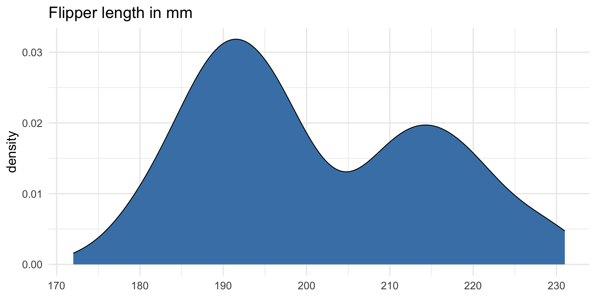
Original vs. mean-centered variable

Original variable

Mean	SD
200.915	14.062

Mean-centered variable

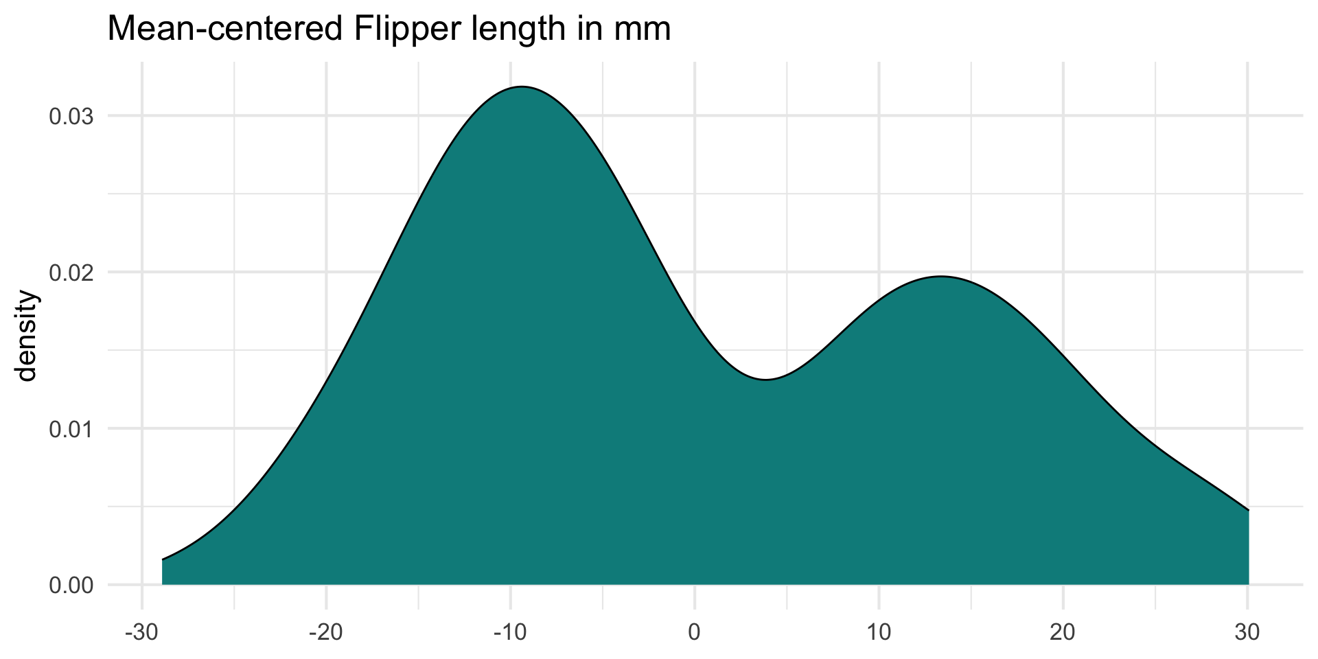
Mean	SD
0	14.062

Using mean-centered variables in the model

How do you expect the model to change if we use flipper_length_cent and bill_length_cent in the model?

term	estimate	std.error	statistic	p.value	conf.low	conf.high
(Intercept)	4318.066	45.674	94.542	0.000	4228.225	4407.908
flipper_length_cent	27.429	3.176	8.638	0.000	21.182	33.675
speciesChinstrap	-748.562	81.534	-9.181	0.000	-908.943	-588.182
speciesGentoo	90.435	88.647	1.020	0.308	-83.937	264.807
bill_length_cent	61.736	7.126	8.664	0.000	47.720	75.753

Original vs. mean-centered model

term	estimate
(Intercept)	-3904.387
flipper_length_mm	27.429
speciesChinstrap	-748.562
speciesGentoo	90.435
bill_length_mm	61.736

term	estimate
(Intercept)	4318.066
flipper_length_cent	27.429
speciesChinstrap	-748.562
speciesGentoo	90.435
bill_length_cent	61.736

What has changed? What is the same?

Standardizing

Standardizing a quantitative predictor mean shifting every value by the mean and dividing by the standard deviation of that variable

\[ X_{std} = \frac{X - \bar{X}}{S_X} \]

Only quantitative predictors are standardized
Standardize all quantitative predictors in the model for ease of interpretation

What is one reason one might want to standardize the quantitative predictors? What is are the units of standardized variables?

Standardizing

Use the scale() function with center = TRUE and scale = TRUE to standardized variables

penguins <- penguins |>
  mutate(flipper_length_std = scale(flipper_length_mm, center = TRUE, scale = TRUE), 
         bill_length_std = scale(bill_length_mm, center = TRUE, scale = TRUE))

Original vs. standardized variable

Original variable

Mean	SD
200.915	14.062

Standardized variable

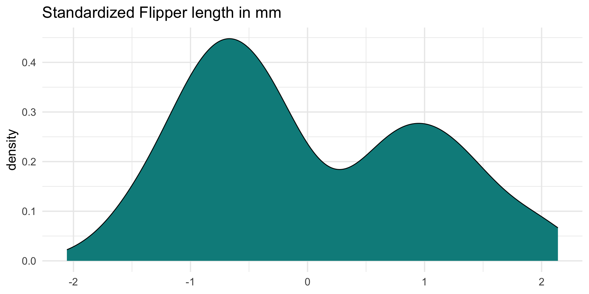
Mean	SD
0	1

Using standardized variables in the model

How do you expect the model to change if we use flipper_length_std and bill_length_std in the model?

term	estimate	std.error	statistic	p.value	conf.low	conf.high
(Intercept)	4318.066	45.674	94.542	0.000	4228.225	4407.908
flipper_length_std	385.696	44.654	8.638	0.000	297.862	473.531
speciesChinstrap	-748.562	81.534	-9.181	0.000	-908.943	-588.182
speciesGentoo	90.435	88.647	1.020	0.308	-83.937	264.807
bill_length_std	337.055	38.902	8.664	0.000	260.533	413.577

Original vs. standardized model

term	estimate
(Intercept)	-3904.387
flipper_length_mm	27.429
speciesChinstrap	-748.562
speciesGentoo	90.435
bill_length_mm	61.736

term	estimate
(Intercept)	4318.066
flipper_length_std	385.696
speciesChinstrap	-748.562
speciesGentoo	90.435
bill_length_std	337.055

What has changed? What is the same?

Interaction terms

Sometimes the relationship between a predictor variable and the response depends on the value of another predictor variable.
This is an interaction effect.
To account for this, we can include interaction terms in the model.

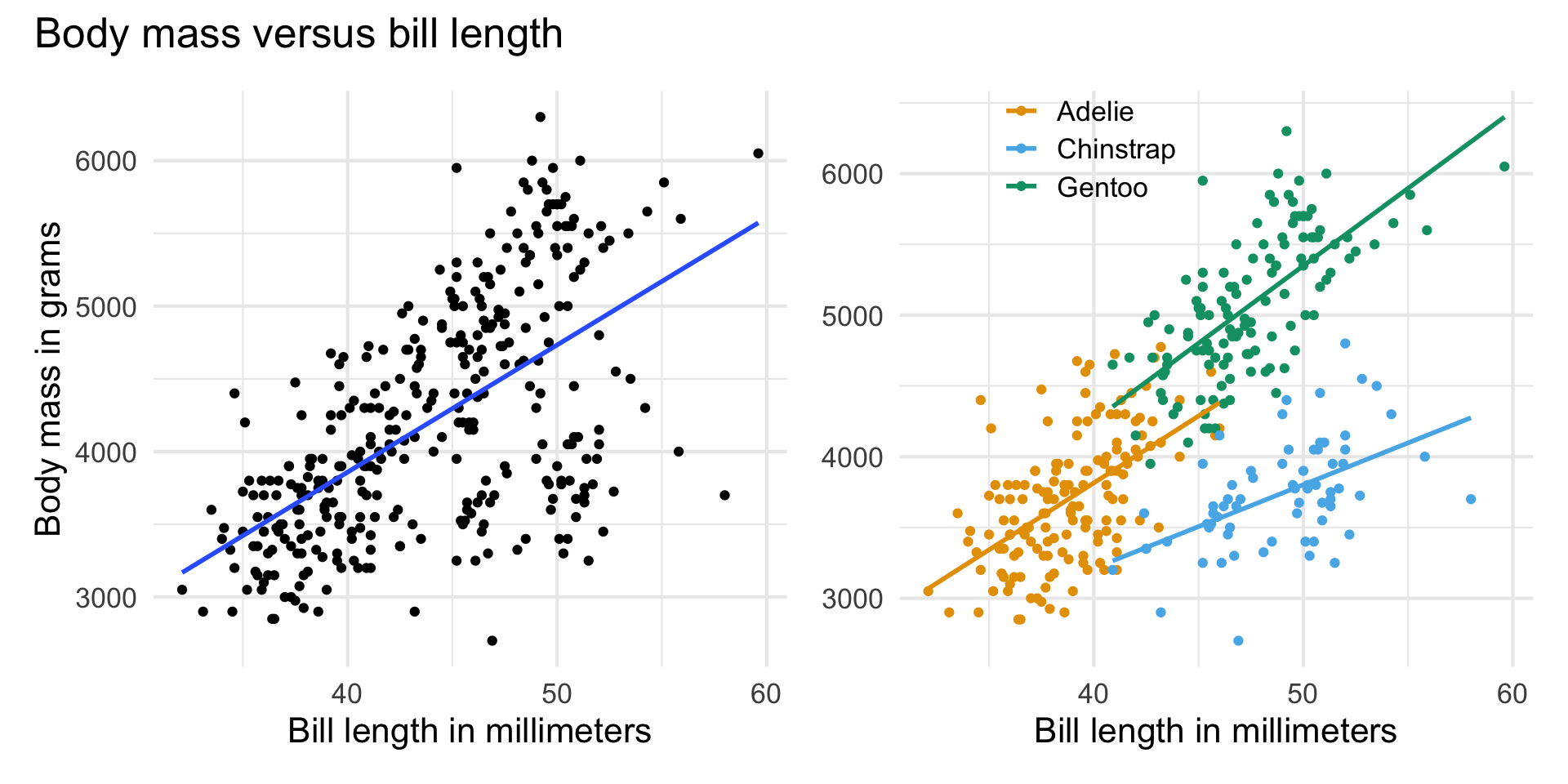
Bill length versus species

If the lines are not parallel, there is indication of a potential interaction effect, i.e., the slope of bill length may differ based on the species.

Interaction term in model

penguin_int_fit <- lm(body_mass_g ~ flipper_length_mm + species + bill_length_mm + species * bill_length_mm,
      data = penguins)

term	estimate	std.error	statistic	p.value
(Intercept)	-4297.905	645.054	-6.663	0.000
flipper_length_mm	27.263	3.175	8.586	0.000
speciesChinstrap	1146.287	726.217	1.578	0.115
speciesGentoo	54.716	619.934	0.088	0.930
bill_length_mm	72.692	10.642	6.831	0.000
speciesChinstrap:bill_length_mm	-41.035	16.104	-2.548	0.011
speciesGentoo:bill_length_mm	-1.163	14.436	-0.081	0.936

Interpreting interaction terms

What the interaction means: The effect of bill length on the body mass is 41.035 less when the penguin is from the Chinstrap species compared to the effect for the Adelie species, holding all else constant.
Interpreting bill_length_mm for Chinstrap: For each additional millimeter in bill length, we expect the body mass of Chinstrap penguins to increase by 31.657 grams (72.692 - 41.035), holding all else constant.

Summary

In general, how do

indicators for categorical predictors impact the model equation?

interaction terms impact the model equation?

Recap

Introduced multiple linear regression
Interpreted coefficients in the multiple linear regression model
Calculated predictions and associated intervals for multiple linear regression models
Mean-centered and standardized quantitative predictors
Used indicator variables for categorical predictors
Used interaction terms

Multiple linear regression (MLR)

Announcements

Computational setup

Considering multiple variables

Data: Palmer penguins

Variables

Response: body_mass_g

Predictors

Response vs. predictors

Multiple linear regression

Multiple linear regression (MLR)

Multiple linear regression

Multiple linear regression

Model fit

Model equation

Interpreting \(\hat{\beta}_j\)

Prediction

Prediction, revisited

Confidence interval for \(\hat{\mu}_y\)

Prediction interval for \(\hat{y}\)

Cautions

Types of predictors

Categorical predictors

Indicator variables

Indicator variables for species

Indicators in the model

Interpreting species

Transforming quantitative predictors

Interpreting the intercept

Centering

Centering

Original vs. mean-centered variable

Using mean-centered variables in the model

Original vs. mean-centered model

Standardizing

Standardizing

Original vs. standardized variable

Using standardized variables in the model

Original vs. standardized model

Interaction terms

Interaction terms

Bill length versus species

Interaction term in model

Interpreting interaction terms

Summary

Recap

Response: `body_mass_g`

Indicator variables for `species`

Interpreting `species`